Chi-Square Test Explained: Counts, Expectations, and Evidence

What a chi-square test asks

A chi-square test compares observed category counts with the counts a null hypothesis predicts. It asks whether the mismatch is unusually large under that hypothesis. It does not tell you the probability that the hypothesis is true, and a small p-value does not by itself explain why a mismatch occurred.

Two common uses are goodness of fit and independence. A goodness-of-fit test compares one categorical variable with specified probabilities, such as equal probabilities for the faces of a die. A test of independence compares two categorical variables in a contingency table, such as course format and completion status. Both use discrepancies between observed and expected counts, but the hypotheses and degrees of freedom differ.

A worked example: 60 rolls of a die

Suppose six categories have observed counts of 8, 9, 10, 11, 12, and 10. These are invented teaching data, not measurements from a real experiment. If the die is fair and rolls are independent, each face has probability 1/6. For 60 rolls, the expected count is 10 in every category.

Face	Observed O	Expected E	(O − E)² / E
1	8	10	0.4
2	9	10	0.1
3	10	10	0.0
4	11	10	0.1
5	12	10	0.4
6	10	10	0.0

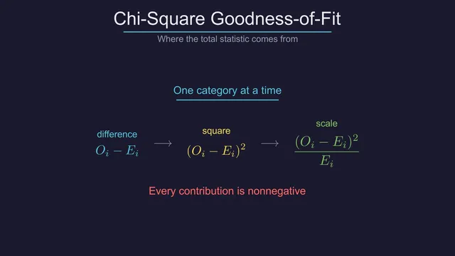
The statistic is χ² = Σ (O − E)² / E = 1.0. Squaring makes discrepancies in either direction contribute positively; dividing by the expected count scales each contribution. The observed bars need not match perfectly even for a fair die. Random variation is exactly why the reference distribution matters.

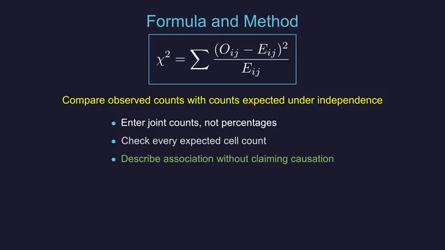
The visual clips illustrate the comparison and formula. They are excerpts from existing animations, not a recording of this worked example. Use the table to follow these particular numbers, and the clips to see the kinds of relationships an animation can expose.

Interpret the statistic using degrees of freedom

Here the six probabilities were specified in advance and no parameters were estimated from the rolls. The reference chi-square distribution has 6 − 1 = 5 degrees of freedom. At a significance level of 0.05, its upper-tail critical value is approximately 11.07. Our statistic of 1.0 is below that threshold, so this example does not reject the fair-die model.

That conclusion is narrower than “the die is fair.” These observations do not provide strong evidence against equal probabilities; they cannot prove exact fairness. The test can miss small departures with limited data. If parameters are estimated from the same sample, the degrees-of-freedom calculation needs an adjustment appropriate to the fitted model. The NIST goodness-of-fit reference explains the test construction and its limitations.

How independence differs

For an r-by-c contingency table, the independence hypothesis predicts each cell count as row total × column total / grand total. Sum the same squared-and-scaled discrepancies across the cells. With the usual conditions and no structural restrictions, the reference distribution has (r − 1)(c − 1) degrees of freedom.

For example, finding an association between course format and completion does not establish that the format caused completion. Students may have selected different formats, or another variable may explain the relationship. The study design determines what you can reasonably conclude after the calculation.

Check the conditions before the arithmetic

Use counts in mutually exclusive, collectively exhaustive categories, with observations independent under the sampling design. Repeated measurements on the same person are not automatically independent. Entering percentages without the underlying sample size loses information needed for the test.

Expected counts, not just observed counts, need to be sufficiently large for the chi-square approximation. A common conservative guideline is at least five expected observations per cell. Sparse tables or rare categories may call for an exact or simulation-based method instead. Do not merge categories only after seeing the result to obtain a preferred p-value; the grouping should make substantive sense.

Make the explanation visible

An effective animation can show the expected bars first, add the observed bars, and then reveal each contribution to χ². Keep the null hypothesis and the meaning of the p-value visible in the explanation. Movement should clarify those steps, not make the result look more certain.

For numerical outcomes compared across groups, read ANOVA explained. The clips on this page were made with LemmaReel; the math animation guide compares ways to build similar teaching material. The calculation above can be understood and checked without buying software.