ANOVA Explained: Between-Group and Within-Group Variation
Work through a one-way ANOVA example, distinguish two sources of variation, and see how the question changes with two factors.
What ANOVA compares
ANOVA means analysis of variance. In a one-way ANOVA, the question is whether population means are equal across groups defined by one factor. The method compares variation between the sample group means with variation among observations inside each group. When the group means are far apart relative to the within-group noise, the evidence against equal population means grows.
For example, imagine comparing scores from three teaching methods. The null hypothesis is that all three population mean scores are equal. The alternative is that at least one mean differs. A significant overall test does not say that every pair differs, identify the best method, or establish that the teaching method caused a difference.
Work through a small example
Use three invented groups for a transparent calculation: A has 2, 3, 4; B has 4, 5, 6; and C has 6, 7, 8. These deliberately small teaching data make the arithmetic easy to inspect; they are not a study or evidence for a teaching intervention.
| Group | Observations | Group mean | Within-group sum of squares |
|---|---|---|---|
| A | 2, 3, 4 | 3 | 2 |
| B | 4, 5, 6 | 5 | 2 |
| C | 6, 7, 8 | 7 | 2 |
The grand mean is 5. The within-group sum of squares is SSW = 2 + 2 + 2 = 6. The between-group sum of squares weights each squared distance from the grand mean by the group size: SSB = 3(3 − 5)² + 3(5 − 5)² + 3(7 − 5)² = 24.
There are k = 3 groups and N = 9 observations. Divide SSB by k − 1 = 2 to obtain a between-group mean square of 12. Divide SSW by N − k = 6 to obtain a within-group mean square of 1. Their ratio is F = 12 / 1 = 12, with numerator and denominator degrees of freedom 2 and 6. Compare that statistic with the appropriate F distribution to obtain a p-value.
For these illustrative numbers, the upper-tail p-value is 0.008. At a preselected 0.05 threshold, the test rejects equal means if its assumptions apply. That is an overall test result, not permission to claim that every pair of groups differs. Report the observed group differences and their uncertainty as well as the p-value.
Why the ratio matters
Imagine increasing the spread of every group while keeping the group means at 3, 5, and 7. The same separation of means would become less distinctive against the noisier observations. Conversely, tightly clustered groups make a difference in means easier to distinguish. This is the intuition behind comparing mean squares rather than simply looking at the largest and smallest mean.
The NIST ANOVA table reference gives the sums of squares, degrees of freedom, and F-test structure. The table above supplies a separate small example you can calculate by hand.
Check the assumptions and the study design
The classical one-way model assumes independent observations, normally distributed errors within groups, and a common error variance. Evaluate these assumptions using the design and suitable residual diagnostics; do not assume they hold just because the software reports a result. With three observations per group, the teaching example is particularly uninformative about the shape of the underlying distributions.
When variances differ, Welch’s ANOVA may be appropriate for independent groups. Repeated measurements, matched participants, or nested classrooms need methods that represent that dependence. A different test is not a substitute for understanding how the data were collected. After an overall rejection, planned contrasts or suitably adjusted pairwise comparisons, such as Tukey HSD when its assumptions are appropriate, can address which differences matter. Effect sizes and confidence intervals help distinguish a detectable difference from a useful one.
One factor versus two factors
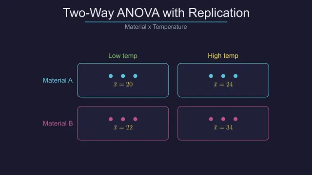
The worked calculation uses one factor: group. Two-way ANOVA considers two factors and can examine whether the effect of one depends on the level of the other. For example, teaching method and practice schedule could have an interaction. An interaction is not simply another name for a large overall mean difference.
The animated grid above illustrates a two-factor layout with cells and group summaries. It is an existing visual excerpt, not the output of the one-way calculation on this page. Keeping that distinction explicit prevents a helpful picture from teaching the wrong model.
Explain the model before presenting a result
A clear lesson should show observations, group means, the grand mean, and the two sources of variation before introducing F. Keep the assumptions and the limits of the conclusion in the narration. For category counts instead of numeric group means, compare the chi-square test explainer. These illustrations were made with LemmaReel; the math animation software guide discusses the production choices behind this kind of lesson.